quick sort python

Overview

In this article I am going to walk through an array sorting algorithm called "Quick sort" in short and clear steps; hopefully to help you understand more how sorting algorithms work in Python in order to enhance your abilities to analyze and solve problems more efficiently.

Before we start

Before we start, you have to know that in order to achieve the best sorting method, and to be able to compare all methods and algorithms together in respect of time and space; Big O is the perfect measure for that.

Big O Notation is a mathematical concept used to describe the complexity of an algorithm as how much time and memory it holds.

Assuming that n is the size of the input to an algorithm, the Big O notation represents the relationship between n and the number of steps the algorithm takes to find a solution.

The following description of some cases will help you understand and classify Big O notation accordingly:

Big O	Complexity	Description
O(1)	Constant	fixed time/space in each time an algorithm is executed.
O(n)	Linear	linearly growth with data size until it reaches O (worst case)
O(n²)	quadratic	directly proportional to square data size "common in nested iterations"
O(2^n)	exponential	double growth with addition of data ex: recursive Fibonacci
O(log n)	logarithmic	little effect on growth while doubling data size

Quick Sort Approach

Just like merge sort, the Quicksort algorithm applies the divide-and-conquer principle to divide the input array into two lists, the first with small items and the second with large items. The algorithm then sorts both lists recursively until the resultant list is completely sorted.

Dividing the input list is referred to as partitioning the list. Quicksort first selects a pivot element and partitions the list around the pivot, putting every smaller element into a low array and every larger element into a high array.

Putting every element from the low list to the left of the pivot and every element from the high list to the right positions the pivot precisely where it needs to be in the final sorted list. This means that the function can now recursively apply the same procedure to low and then high until the entire list is sorted.

Pseudocode

The next Pseudocode shows how to implement the Quick sort algorithm:

ALGORITHM QuickSort(arr, left, right)
    if left < right
        // Partition the array by setting the position of the pivot value
        DEFINE position <-- Partition(arr, left, right)
        // Sort the left
        QuickSort(arr, left, position - 1)
        // Sort the right
        QuickSort(arr, position + 1, right)

ALGORITHM Partition(arr, left, right)
    // set a pivot value as a point of reference
    DEFINE pivot <-- arr[right]
    // create a variable to track the largest index of numbers lower than the defined pivot
    DEFINE low <-- left - 1
    for i <- left to right do
        if arr[i] <= pivot
            low++
            Swap(arr, i, low)

     // place the value of the pivot location in the middle.
     // all numbers smaller than the pivot are on the left, larger on the right.
     Swap(arr, right, low + 1)
    // return the pivot index point
     return low + 1

ALGORITHM Swap(arr, i, low)
    DEFINE temp;
    temp <-- arr[i]
    arr[i] <-- arr[low]
    arr[low] <-- temp

Lets assume the input of our algorithm is the following array/list:

array = [8, 2, 6, 4, 5]

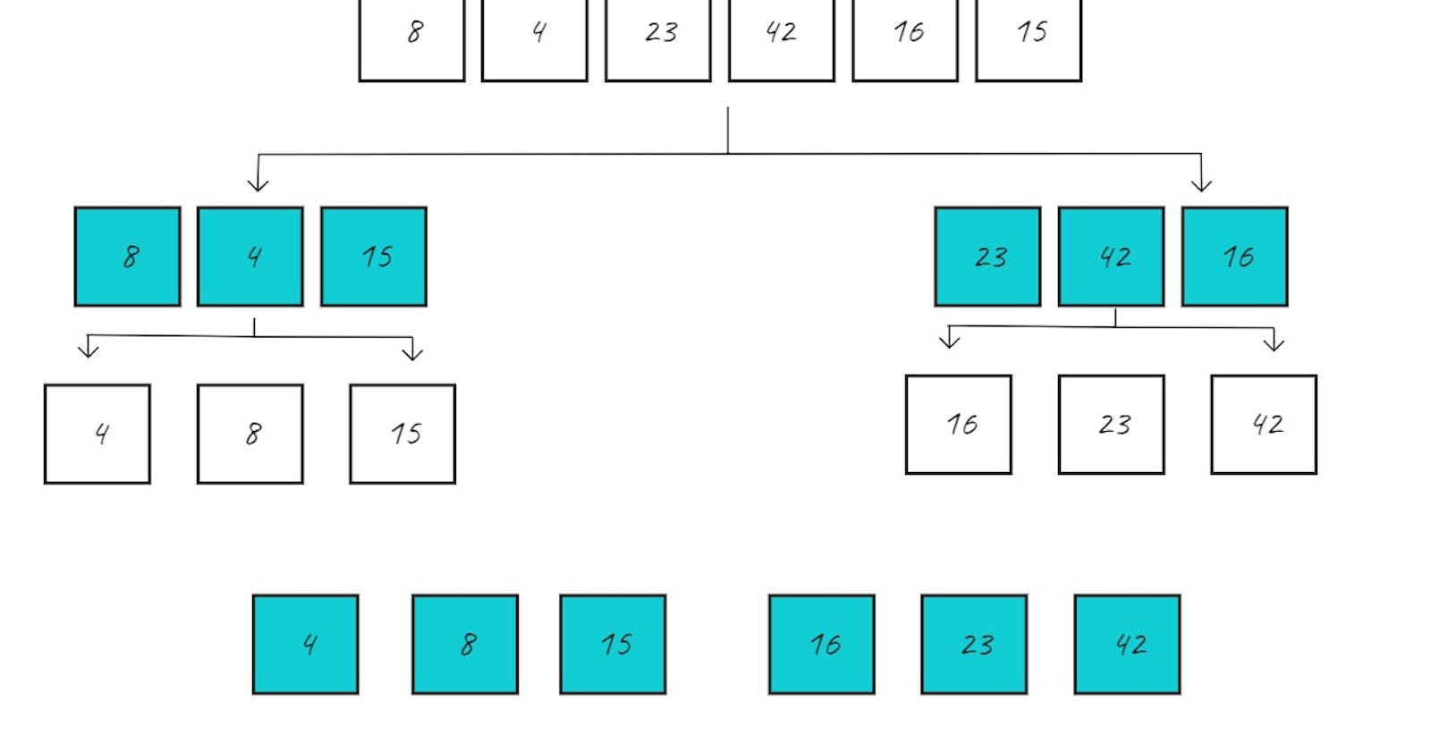
To make it more clear and easy to understand, here is a step-by-step visualization of each algorithm iteration for the array:

Quick Sort.jpg

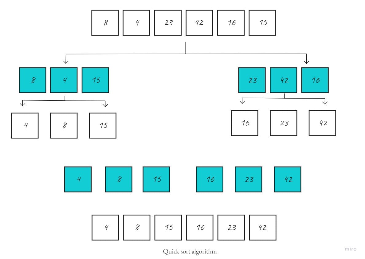
As you can see, the array is supposed to be sorted ascendingly by splitting the original array into two parts, then recursively dividing the parts until the result array reaches a total number of elements.

Algorithm

Now, lets review the steps of solving this problem so we can implement it using Python: The pivot element is selected randomly. In this case, pivot is 6.

The first pass partitions the input array so that low contains [2, 4, 5], same contains [6], and high contains [8].

quicksort() is then called recursively with low as its input. This selects a random pivot and breaks the array into [2] as low, [4] as same, and [5] as high.

The process continues, but at this point, both low and high have fewer than two items each. This ends the recursion, and the function puts the array back together. Adding the sorted low and high to either side of the same list produces [2, 4, 5].

On the other side, the high list containing [8] has fewer than two elements, so the algorithm returns the sorted low array, which is now [2, 4, 5]. Merging it with same ([6]) and high ([8]) produces the final sorted list.

Code Implementation

Here is the implementation of Python code for Quick sort approach, built upon the algorithm steps above:

     from random import randint

def quicksort(array):
    if len(array) < 2:
        return array

    low, same, high = [], [], []
    pivot = array[randint(0, len(array) - 1)]

    for item in array:
        if item < pivot:
            low.append(item)
        elif item == pivot:
            same.append(item)
        elif item > pivot:
            high.append(item)

    return quicksort(low) + same + quicksort(high)

Big O Notation

In Quick sort the input list is partitioned in linear time, O(n), and this process repeats recursively an average of log2n times. This leads to a final complexity of O(n log2n).

Source Code

GitHub

Diala's Blog

Diala's Blog

Quick Sort Algorithm

Step-By-Step With Python

Table of contents